Practical Approach to the Ecosystem Modeling
Marine ecosystem comprised of microscopic life to top predators that provide resources and services which are key to the health and wellbeing of human society. Coastal areas are generally rich in marine ecosystems and biodiversity as well as centers of economic activities including fishing, shipping, mariculture, tourism, and recreation, etc. so predicting these ecosystem states on sub-seasonal to interannual timescale is getting top priority.
Understanding and quantitatively describing marine ecosystems requires the integration of physics, chemistry, and biology. Coupling biology and physical oceanography in models has many attractive features. We can do experiments with models of marine systems while the real system can only be observed in the state at the time of the observation. We can also employ the predictive potential of models for applications such as environmental management or experimental simulations.
The ecosystem modeling is the mathematical representation of ecological systems ranging from individual population to entire biome which is studied to better understand and prediction about the dynamics of the real ecosystem. More specifically, ecosystem models are a computer that consists of algorithms that represents a set of important ecological processes to compute ecosystem dynamics over time.
Ecosystem models can be characterized roughly by their complexity for example by the number of state variables and the degree of process resolution.
Models enable researchers to simulate large scale over a very long period’s experiments that would be costly in the real world. Ecosystem modeling requires the combination of both the biological and the physical system. The physical feature of a system shapes the potential range of the chemical-biological developments. Obvious examples of physical determinants are the yearly cycle and range of temperature, typical mixing, depths, and vertical stratification as well as transport and distribution of nutrients due to advection and turbulent diffusion. Inhomogeneous physical forcing provides scales that need to be resolved in models for many applications. Strong spatial gradients in the biogeochemical variables also require adequate spatial resolution.
Modeling variables
General ecosystem models have three types of variables
1: state variables: state variables represent various ecological entities, attributes, or characteristics with values that change during the simulation. Common state variables are carbon, the concentration of nutrients, biomass, and abundance. The dynamics of the state variables are driven by processes such as nutrient uptake, respiration, and grazing as well as physical processes such as light variations, turbulence, and advection. The state variables are influences by various ecosystem flows (flux variables) that cause increases and decreases in the state variables and these flow represent ecosystem processes. For example nitrogen loss via decomposition. The computation of simulated fluxes and how they change state variables almost always require intermediate variables which are variables used to determine transitional products within the algorithm. And last, there are many types of output variables that are written to computer files for later analysis. Response variables are those output variables that used to directly answer the modeling project’s objective and explanatory variables are used to explore and explain behaviors of the response variables. Diagnostic variables are used to explore model behavior while changing a specific parameter, processes, or algorithm in the various phases of a modeling project. Each modeled flux or process is usually represented by a coded equation that always has a constant or dynamic parameter which are values that quantify coefficients or threshold values in that algorithms. Values for static parameters are set within the computer code and the user often cannot change these values but dynamic parameters are usually input into the model by the user. The computer model often reads values for input variables which can be parameters or initial values. Initial values are the quantification of the starting value of a state, intermediate, or flux variables.

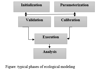
Major phases of the modeling
1: initialization: initialization is the process of quantifying the initial conditions that form the starting place for model simulation.
2: parameterization: parameterization is the quantification of the parameters need by model algorithms. It is a preliminary modeling phase that is absolutely required in all modeling projects (Grimm and Railsback 2013). This step will not only quantify the information needed to run the model but also it will help the user understand the model and the algorithms that comprise the model. Poor parameterizations are major problems in many modeling projects (Jakeman et al. 2006).
Five major methods are often used to quantify model parameters and they involve estimating from the following sources
a. Field measurements. The site, water, plant, and animal characteristics can be measured in the field to quantify parameters in the model.
b. Existing data syntheses.
c. Literature searches.
d. Iterative model approximations.
e. Expert opinions.
Each of these methods has advantages and disadvantages.
3: calibration: calibration is the adjustment of model parameters to increase realism. Calibration performs many important tasks the user (1) develops a solid feel for model behavior from the iterative runs, (2) becomes confident in interpretation results, (3) detects obvious problems with initialization and parameterization, (4) learns the sensitivities of model parameters and (5) prepares the model for the execution of the project.
4: validation: validation is the estimation of the accuracy and precision of model results. Calibration usually occurs after most parameters and initial conditions are quantified. Once the model is calibrated, then it is possible that the modeling project, is ready for execution but an estimate of model uncertainty is often needed to evaluate and interpret model results. Validation requires simulated output to be compared against measured data to determine accuracy.
5: execution: execution is the process of actually running the model to complete the simulation design of the modeling project
6: analysis: analysis is the process of synthesizing and summarizing model results to complete the modeling project and answer the modeling object. Analysis usually involves importing the simulated data into a data management system such as spreadsheets or databases and then linking to the statistical program to perform advanced statistical and graphic analysis.

Ecosystem models have a wide range of applications such as natural resource management, ecotoxicology, environmental health, agriculture, and wildlife conservation.
The most common ecosystem model is lotka and Volterra which is known as the predator-prey model of Alfred J. lotka (1925) and vito volterra (1926)

X is the number/concentration of the prey species;
Y is the number/concentration of the predator species;
is the prey species’ growth rate;
is the predation rate of Y upon X;
is the assimilation efficiency of Y;
is the mortality rate of the predator species
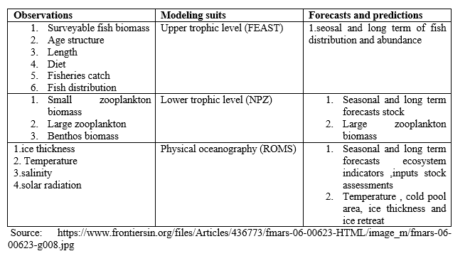
NPZ (the nutrient phytoplankton zooplankton) model is a common tool in oceanographic research. The NPZ model incorporates one of the simplest sets of dynamics that usefully describe oceanic plankton dynamics. The state variables for this model include nutrient (N), plankton (P), and zooplankton (Z). These are usually modeled in terms of their nitrogen content since nitrogen is often limiting to primary production in the ocean.

In nature, the aquatic ecosystems consist of individuals (copepod, fish) that have biomass and form populations.
Ecosystem modeling is an interdisciplinary task that required a well-balanced dialogue of biologists and modelers to address the right questions and to develop theoretical descriptions of the processes to be modeled. Models are mathematical tools by which we analyze, synthesize, and test our understanding of the dynamics of the system through retrospective and predictive calculations.
To reduce the complexity of nature with models. There are several models types
1. Models of individuals: the individual-based models consider individuals as basic units of the biological system while state variable models look at numbers or mass of very many individuals per unity of volume.
2. Populations models: the fish population is considered as the sum of individuals whose dynamics are controlled by growth, mortality, and recruitment. Some knowledge of the life cycle of fish is usually taken into account.
3. Biomass models
4. Combined individuals and populations models
5. Models combining aspects of populations, biomass, and individual dynamics
The reasons include
1. To develop and enhance understanding
2. To quantify descriptions of processes
3. To synthesize and consolidate our knowledge
4. To establish the interaction of theory and observation
5. To develop predictive potential
6. To simulate scenarios of past and future developments

Some existing ecosystem models
1: Ecopath
2: StrathE2E
3: BFM
4: ERSEM
5: SHYFEM
6: MEDUSA (model of ecosystem dynamics, nutrient utilization, sequestration, and acidification) is an intermediate complexity model of lower trophic level ecosystem run within a global earth model to address biogeochemical response to anthropogenic drivers.
Ecological resources and associated ecosystem services are key components of the blue economy and continued monitoring across multiple levels of biological organization and ensuring sustainable development.
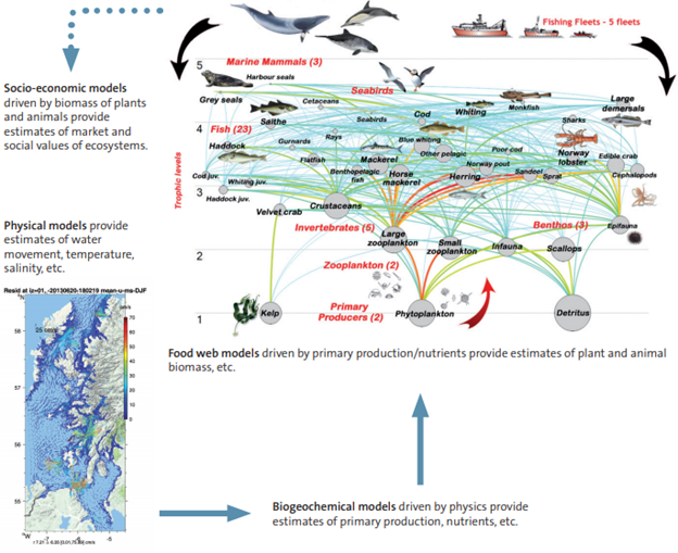
Modeling the marine ecosystem requires an integrated approach that involves biogeochemical processes, food web interaction, and the control of these processes by the physical environment. Monitoring biodiversity and ecological patterns improve our understanding of ecosystem dynamics and support conservation and management planning.
Marine ecosystem models are an important analytical approach to integrate knowledge, data, and information, improve understanding of an ecosystem's functioning, and complement monitoring and observation efforts. They also offer the potential to predict the response of the marine ecosystem to future scenarios and to support the implementation of ecosystem-based management of our seas and ocean. Additionally, ecological observations and modeling can provide essential input to physical or biogeochemical models and inspire alternative modeling approaches.
Modeling Tools:
1: Marine Geospatial Ecology Tools (MGET)
MGET is an open-source geoprocessing toolbox that can solve a wide range of marine research, conservation, and spatial planning problems. You can use it within ArcGIS [10.1 -10.5].
2: Ecopath with Ecosim : Ecopath with Ecosim is a free and open-source ecosystem modeling software suite, initially started at NOAA by Jeffrey Polovina, but has since primarily been developed at the formerly UBC Fisheries Centre of the University of British Columbia.
References
1: https://www.terrapub.co.jp/journals/JO/pdf/5802/58020379.pdf
2: apply ecosystem and landscape models in natural resources management
3: https://www.ecologycenter.us/population-dynamics-2/marine-ecosystem-modeling-approaches.html
4: https://www.frontiersin.org/articles/10.3389/fmars.2019.00623/full
